Random Variables and its Probability Distributions

 

Table of Content

What is a Random Variable? Types of Random Variable Discrete Random Variable Continuous Random Variable Probability Mass Function What is Probability Distribution? Cumulative Distribution Function (C.D.F) of Discrete Random Variable Problems Probability Density Function Distribution Function

What is a Random Variable?

A Random Variable or Stochastic Variable or Random quantity in the field of probability and statistics is a variable quantity, whose possible values depend on a set of random outcome events in random manner.

The outcome space is defined in terms of set theory or a set.

A random variable is a function associating a real number with each outcome of a sample space S of a random experiment and it is denoted by X.

Domain of a random variable X is a sample space S and codomain or range of a random variable X is the set of real values taken by X, Thus, symbolically X: S-> R.
 

Types of Random Variable

There are two types of Random Variable:

• Discrete Random Variable

• Continuous Random Variable

Discrete Random Variable

A random variable X which can assume countable number of isolated values (integers) is called discrete random variable. The meaning of the word ‘discrete’ is separate and individual

Examples:

• Number of kids in a family

• Number of attempts to hit a target

• Number of heads in tossing a coin thrice

• Number of stars in the sky
   

Continuous Random Variable

A random variable X which can assume all real values within a given interval is known as continuous random variable. Thus, the possible values of a continuous random variable are uncountably infinite.

Examples:

• Price of a commodity

• Age of a person

• Height of a person in cm

• Life of an electric component (in hours)
   

Examples to identify random variables as either discrete or continuous in each of the following situations:

Q1.  A  page in a book can have at most 300 words

X= Number of misprints on a page

Solution

X = Number of misprints on a page

Since a page in a book has at most 300 words, X takes the finite values

Therefore, random variable X is discrete

Range = {0, 1, 2….299, 300}
 

Q2. A gymnast goes to the gymnasium regularly

X = Reduction of his weight in a month

Solution

X = Reduction of weight in a month

X takes uncountable infinite values

Therefore, random variable X is continuous.
 

Probability Mass Function

If X is the discrete random variable taking values x₁, x₂, x₃…x_n and we find the values of P(X = x₁), P(X = x₂), P(X = x₃)…P(X = x_n), then we obtain the functions P(x) = P(X = x) for x = x₁, x₂, x₃…x_n.

This function is called Probability Mass Function (p.m.f) of the random variable X.

Example

If two coins are tossed and X=number of heads, then the sample space of tossing two coins is {HH, HT, TH, TT}

Therefore, P(X = 0) = P (0) =1/4, P(X = 1) = P(1) = 2/4 = 1/2

P(X = 2) = P (2) = 1/4

Hence, the probability mass function is given by

P(x) = 1/4, x = 0

=1/2, x = 1

= ¼, x = 2

For the sample space S = {0, 1, 2} for X.

Note:

If X is any random variable taking values from sample space S and P(x) is the probability mass function of X such that x ∈ S, then

• 0 ≤ P(x) ≤  1 for all x ∈ S

• ∑ P(x) = 1, that is, the total of all values of P(x) for x ∈ S is always unity.

We can verify this in the example given above

∑ P(x) = P(0) + P(1) + P(2) = 1/4 + 1/2 + ¼ =1
 

What is Probability Distribution?

If X is a discrete random variable taking values x₁, x₂, x₃….x_n with corresponding probabilities p₁, p₂, p₃…p_n, then the set of ordered pairs (x_i, p_i), i = 1, 2, 3….n is called a Probability Distribution of the random variable X.

Example

If the two coins are tossed and X is the number of heads, then the probability distribution of the random variable X can be given as below:

X	0	1	2
P(X)	¼	4-Feb	4-Jan

Note that the sum of all probabilities

 = ¼ + 2/4 + ¼ = 4/4 = 1

In general case, the probability distribution of discrete random variable X can be given as:

X	X1	X2	X3	….	Xn
P(X)	P1	P2	P3	….	Pn

Where ∑ p_i = p₁ + p₂ + p₃ +….+ p_n = 1
 

Cumulative Distribution Function (C.D.F) of Discrete Random Variable

Let X be a discrete random variable and its probability distribution is as follows:

X = xi	X1	X2	X3	…	Xn	Total
Pi = P[X = xi]	P1	P2	P3	…	Pn	1

The Cumulative Distribution Function (c.d.f) of X is denoted by F(x) and it is defined as

F(x) = P[X ≤ x], x ∈ R

Notes:

• Domain of c.d.f is R

Codomain of c.d.f is [0, 1]

• F(x_i) = P[X ≤ x_i] = p₁ + p₂ + p₃ +….p_i, i = 1, 2, 3,…n

• c.d.f of a discrete random variable X is also represented in tabular form as follows:

X=xi	F(xi)
X1	P1
X2	P1+P2
X3	P1+P2+P3
…….	…….
Xn	P1+P2+P3+…..+Pn

• C.D.F. is often called Distribution Function (D. F)
   

Problems

Q1. Three balanced coins are tossed simultaneously. If X denotes the number of heads, find probability distribution of X.

Sol.  When three balanced coins are tossed then the sample space is

{HHH, HHT, HTH, THH, HTT, THT, TTH, TTT}

X denotes the number of heads.

X can take the values 0, 1, 2, 3

P[X = 0] = P (0) = 1/8
P [X = 1] = P (1) = 3/8

P[X = 2] = P (2) = 3/8
P [X = 3] = P (3) = 1/8

Q2. Given below is the probability distribution of X:

X	0	1	2	3	4
P [X= x]	k	2k	4k	2k	k

• Find the value of k

• P (X ≥  2), P(X < 3 ), P(X≤1)

• Obtain the c.d.f of X

Solution:

• Since P(X) is the probability distribution of X,

∑ P[X = x] =1

P[X = 0] + P[X = 1] + P[X = 2] + P[X = 3] + P[X = 4] = 1

k + 2k + 4k + 2k + k =1

10k = 1

k = 1/10

• P (X ≥ 2) = P[X = 2] + P[X = 3] + P[X = 4]

= 4k + 2k + k = 7k

= 7 (1/10) = 7/10

P (X<3) = P[X=0] +P [X=1] + P[X=2]

= k + 2k+ 4k = 7k

= 7 (1/ 10) = 7/10

P (X≤ 1) = P[X=0] + P [X=1]

= k +2k = 3k

= 3 (1/10) = 3/10

• By definition of C.D.F,

F(x) = P (X ≤ x)

F(0) = P (X ≤ 0) = P(0) = k = 1/10

F(1) = P(X ≤ 1) = P(0) + P(1) = k + 2k = 3k = 3/10

F(2) = P(X ≤ 2) = P(0) + P(1) + P(2) = k + 2k + 4k = 7k = 7/10

F(3) = P(X ≤ 3) = P(0) + P(1) + P(2) + P(3) = k + 2k + 4k + 2k = 9/10

F(4) = P(X ≤ 4) = P(0) + P(1) + P(2) + P(3) + P(4) = k + 2k + 4k + 2k + k = 10/10 = 1

Hence, the c.d.f of X is as follows:

xi	0	1	2	3	4
F(xi)	10-Jan	10-Mar	10-Jul	10-Sep	1

Probability Density Function (P. D. F) and Distribution Function (D. F) of a Continuous Random Variable
 

Probability Density Function

  A real valued function f(x) is called a Probability Density Function (P. D. F) of a continuous random variable X, if it satisfies the following:

• F(x) ≥ 0 for all x ∈ R

Notes:

• If X takes the values in the interval (a,b) then the function f(x) is such that

  • F(x) ≥ 0 for a < x <  b, and

  • ∫^b_a    f(x) dx =1

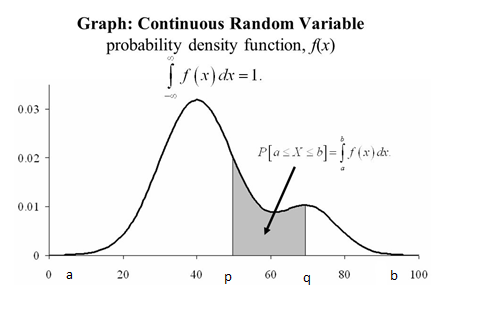
• The geometrical representation is as below:

The area under the curve y= f(x) bounded by the X-axis and the coordinates x = a and x = b is 1, because it represents the total probability P(a< X <b) which is equal to 1.

Also, P (p < X < q) is area under the curve y = f(x) bounded by the X-axis and the coordinates x = p and x = q which is shaded in the figure.

The graph of the P. D. F of R. V. X is called the Probability Curve or Probability Density Curve.
 

Distribution Function

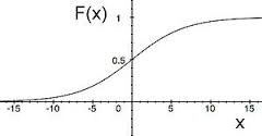
Assume X as a continuous random variable with probability density function f(x), then the cumulative distribution function F(x)of X is defined for every real number x_i, as F(x_i) =P [X ≤ x_i] = ∫ f(x) dx

Remarks:

• F(x_i) is the area under the curve y= f(x) to the left of x as shown in the figure right:

• F(x) increases smoothly as x increases

• If range of X is (a,b) then F(x) = 0, for x< a and F(x) = 1, for x≥b

• P [X >x]=1 - P [X ≤ x_i]= 1- F(x)
   

More Readings

Random Variables and its Probability Distributions